General motion

Solid State Physics

Properties of electrons

Unit 2: Electronic Structure of Atoms

https://www.youtube.com/watch?v=EMq_QbyghMU

Particle in box是量子力学经典模型，涉及解决Time-Independent Schrodinger Equation：

$$-\frac{\hbar^2}{2m}\frac{\partial \varphi}{\partial x^2}=E\varphi$$

Unit 3: Bonding Between Atoms

Unit 4: Crystal

常识性的：

4.1 Motifs and Lattices

• 2D Bravais Lattices

总的来说，二维的布拉维格子可以归纳为4种:

在这四种shape以外的，都无法通过平移填满整个二维平面，因此无法作为valid unit cell.

• 3D Bravais Lattices

三维晶体必然由某种粒子按照以上七种bravais lattices形成motif，即unit cell.

当atom只分布在corner上时，这种unit cell，被称为是’primitive’的，而fcc，bcc此类不仅仅在corner上有原子的晶胞，就属于non-primitive. 原子不能随意分布，基于七种基本的primitive bravais lattices结构，一共有十四种bravais lattices.

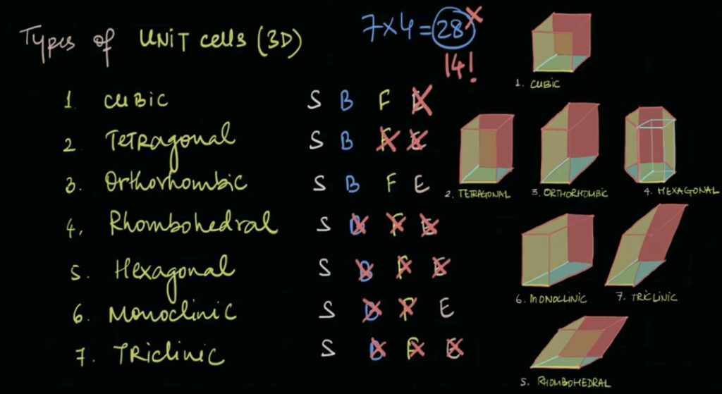
整理后如下，可以清晰看到衍生关系：

常见问题

如何判断一个二维点阵是否为布拉维晶格？

判断依据是点阵中所有点的环境是否相同.

若二维点阵中每一个点的周围环境（包括相邻点的数量、距离和排列方式等）都完全一致，即通过平移矢量 $\vec{T} = n\vec{a} + m\vec{b}$,（n, m 为整数）平移后，所有点的环境不变，则该二维点阵为布拉维晶格；若存在至少两个点的环境不同（如相邻点的数量、距离或排列有差异），则不是布拉维晶格.

---

一个晶格点上只能有一个原子吗？

一个晶格点上不一定只有一个原子.

一个晶格点（Lattice Point）是为了描述晶体周期性而引入的抽象几何点，并非实际原子，因此晶格点上可以没有原子，也可以有多个原子；例如，在一些复杂晶体结构中，一个晶格点可能对应一个基元（Motif），基元可包含多个原子.

---

有其他原子，不妨碍某种原子是布拉维晶格吗？

不妨碍.

布拉维晶格关注的是晶格点的周期性和每个晶格点环境的一致性，而非具体原子种类。即使存在其他原子，只要某种原子的排列方式满足：所有晶格点的环境相同（通过平移矢量 $\vec{T} = n\vec{a} + m\vec{b}$ 重复后，原子排列的相对关系不变），则这种原子的排列可构成布拉维晶格。例如，在 $\ce{NaCl}$ 结构中，虽然存在 $\ce{Na+}$ 和 $\ce{Cl-}$，但面心立方（FCC）的晶格点（顶点和面心）环境一致， $\ce{Na+}$ 或 $\ce{Cl-}$ 的排列均可基于此晶格描述，其他原子的存在不影响晶格本身的布拉维性质。

综上，晶格点与原子数量无必然限制关系，其他原子的存在也不影响某种原子的排列构成布拉维晶格，关键在于晶格点的周期性和环境一致性.

Planes in Lattices

Unit 5: Diffraction

Reference：https://www.youtube.com/watch?v=4JjhiyXcPl8

5.1 衍射的基本原理 – Huygens-Fresnel principle

Diffraction is the bending of a wave due to interference with an object.

光遇到障碍物时，我们观察到它会发生弯曲，我们用Huygens principle解释这个现象

空间中到处都有光的ether particles，无时无刻不在振荡，在wavefront上的每一个ether particle都会产生它们的次级波；换言之，wavefront上的每个点都充当一个新的source，产生一个新的spherical wave（球面波，即secondary wave），而所有点的所有次级波可以找到一个共同的envelope line，这就是新的wavefront：

Diffraction effects most noticeable when size of obstacle is ~ to wavelength.

5.2 Diffraction from a Lattice

• X-ray Diffraction (XRD)

X-ray在大多数情况下与lattice发生destructive interference（相消干涉），但在特定角度下可发生constructive interference（相长干涉）

• Systematic absence

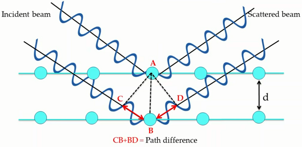
• Bragg’s Law

发生constructive interference的必要条件：

$$n\lambda =2d\sin\theta$$

5.2 Structure Factors

Unit 6: Mechanical Properties

6.1 Stress and Strain

• Stress

$$ \sigma=\frac{F}{A} $$

• Strain

$$ \varepsilon_{true} =\frac{dx}{x} $$

6.2 Stress-Strain Curve

• Elastic Regime

For most of this regime, stress and strain are proportional:

$$ \sigma=E\varepsilon $$

• Young’s Modulus

6.3 Dislocations

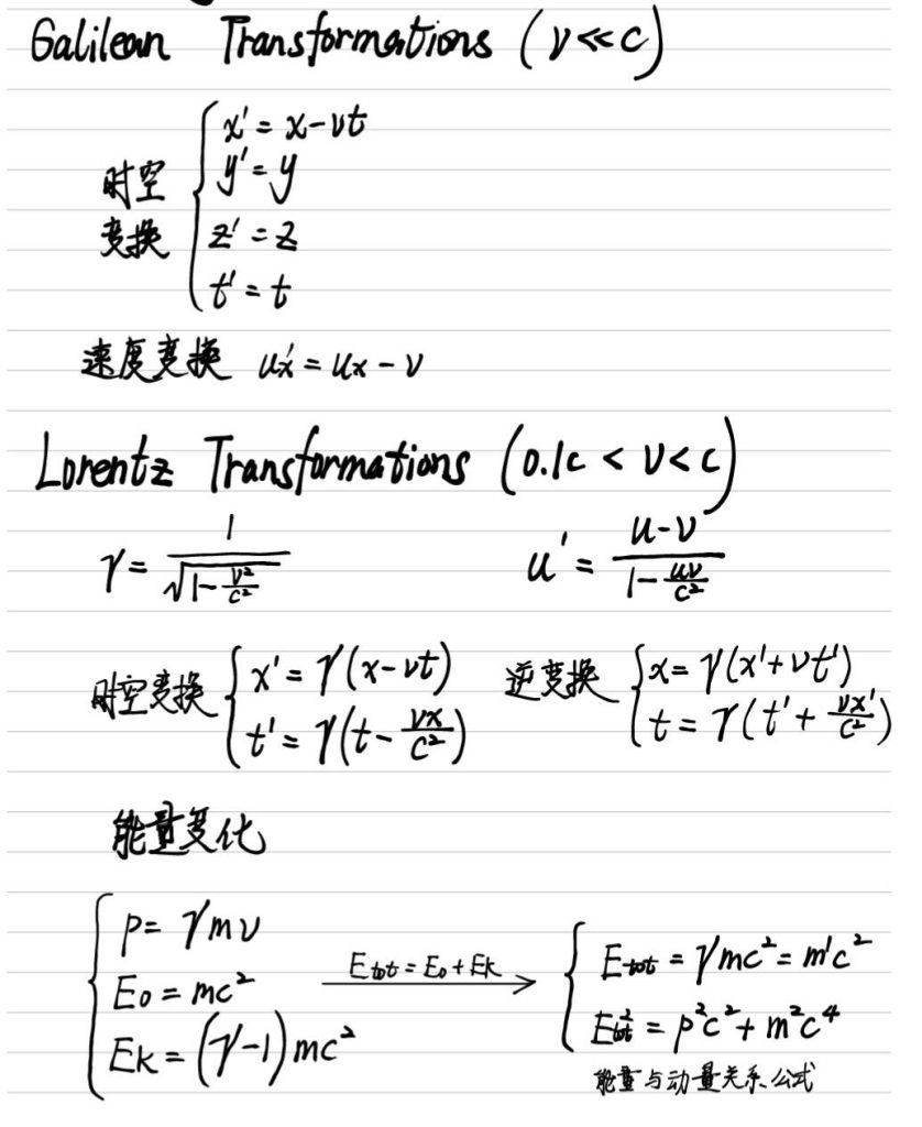
Special Relativity

The role of relativity, in physics, is to study how that motion looks from different perspectives.

一个物品在空间中的位置取决于point of reference，即坐标系的选取：

坐标系的移动

从静止的角度看运动，位置是相对的，距离的比率是绝对的.

https://www.youtube.com/watch?v=hTxWAQGgeQw

平移

$$x_{new}=x-\Delta x$$

$$y_{new}=y-\Delta x$$

旋转

$$x_{new}=x\cos\theta-y\sin\theta$$

$$y_{new}=y\cos\theta+x\sin\theta$$

Lorentz Transforms

length contraction

Thermodynamics

Enthalpy

Sublimation

升华过程的焓变是熔化（fusion）和汽化（vaporization）焓变之和：

$$\Delta_{\text{sub}}H^{\ominus} = \Delta_{\text{fus}}H^{\ominus} + \Delta_{\text{vap}}H^{\ominus}$$

Hess’s law

化学反应的总焓变与反应途径无关，只要反应的起始状态（反应物）和最终状态（生成物）相同。这是因为焓（$H$）是状态函数，反应的焓变（$\Delta_r H$）仅取决于系统终态（产物）与初态（反应物）的焓差，与中间步骤或反应路径无关；热化学方程式可像代数方程一样进行加减、乘以常数等运算。例如，将分步反应的方程式相加（同时焓变相加），消去中间产物，即可得到总反应及其焓变.

一般反应焓变公式

$$\Delta_{r}H_{298}^{\ominus} = \sum \underbrace{\nu_{i}\Delta_{f}H_{298}^{\ominus}(产物)}_{\text{所有产物标准生成焓变之和}} – \sum \underbrace{\nu{i}\Delta_{f}H_{298}^{\ominus}(反应物)}_{\text{所有反应物标准生成焓变之和}}$$

其中 $\nu_{i}$ 是化学计量系数（stoichiometric coefficient），焓是广度性质（extensive quantity），传热与物质的量有关.

一般反应示例

对于 $\alpha A + \beta B \to \gamma C + \delta D$，

$$\Delta_{r}H_{298}^{\ominus} = [\gamma\Delta_{f}H_{298}^{\ominus}(C) + \delta\Delta_{f}H_{298}^{\ominus}(D)] – [\alpha\Delta_{f}H_{298}^{\ominus}(A) + \beta\Delta_{f}H_{298}^{\ominus}(B)]$$

Enthalpy changes of combustion $\Delta_c H^{\ominus}$

• $\Delta_c H^{\ominus}$ 是 1 mol 物质在 1 bar 压力下与氧气完全反应时的焓变，数值通常在 298K 下给出。标注 298K 表示反应物从 298K 开始，产物也在该温度结束；虽然燃烧过程中温度会升高，但关键在于起始和结束温度

• 燃烧焓变总是负值（always negative values），因为燃烧总是放热（gives out heat）；计算时必须包含负号，以确保算术运算正确

Enthalpy changes of solution $\Delta_{sol} H^{\ominus}$

1 mol 物质在1 bar 压力下溶于大量溶剂时的焓变

焓变和溶剂量无关

Kirchhoff equation

$$H_{T_2} = H_{T_1} + C_p \Delta T$$

其中，$\Delta T = T_2 – T_1$

对于 1 mol 物质，温度从 $T_1$ 变化到 $T_2$ 时，焓从 $H_{T_1}$ 变为 $H_{T_2}$，变化量由恒压热容 $C_p$ 和温度变化 $\Delta T$ 决定

若已知温度 $T_1 $ 时反应的焓变 $ \Delta H_{T_1} $，则另一温度 $T_2 $ 时的 $ \Delta H_{T_2} $ 可通过反应物和产物的焓随温度变化推导（即Kirchhoff equation）：

$$\Delta H_{T_2}^\ominus = \Delta H_{T_1}^\ominus + \Delta C_p (T_2 – T_1) $$

其中 $ \Delta C_p $为反应中产物与反应物热容的差值（$ \Delta C_p = C_{p,产物} – C_{p,反应物} $）

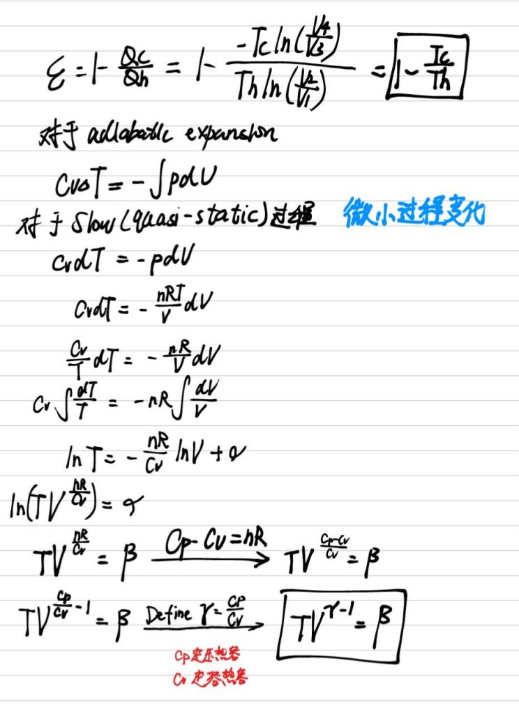
Carnot Circle

Heat engine

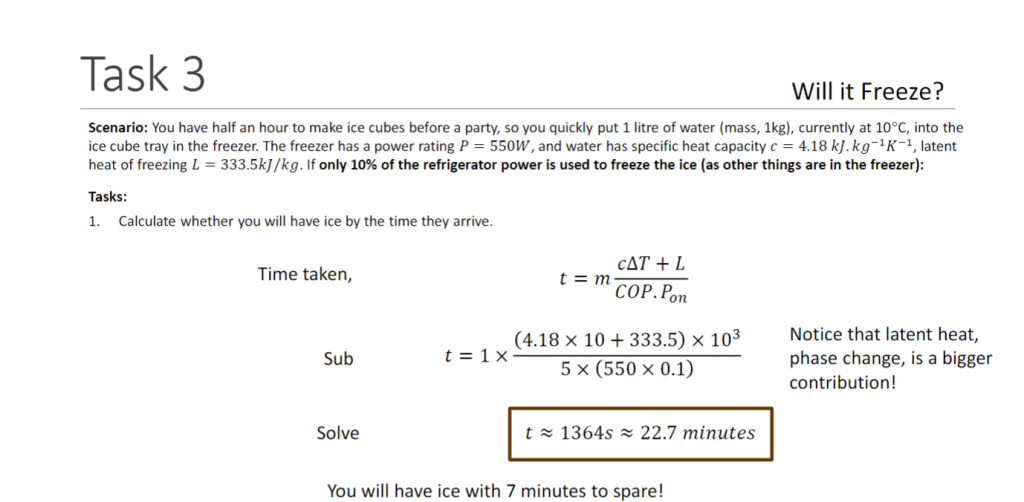
可逆热机 Reversible engine

可逆热机是可以进行可逆循环的热机，既能从高温热源$T_h$吸热，在低温热源$T_c$放热，完成一个循环；也能逆着该循环，从低温热源$T_c$吸热，在高温热源$T_h$放热；每一个步骤都是可逆的，即过程可无限缓慢（准静态）进行，系统始终处于热力学平衡状态.

$$\eta=1-\frac{T_c}{T_h}$$

在两个给定热源之间工作的任何热机，其效率都不会高于在这两个热源之间工作的可逆热机.

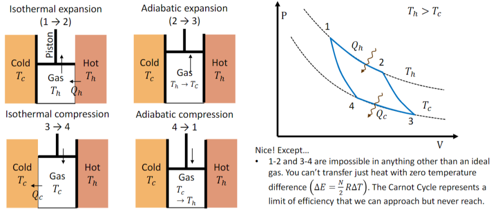
Detailed process

• isothermal expansion
• adiabatic expansion
• isothermal compression
• adiabatic compression

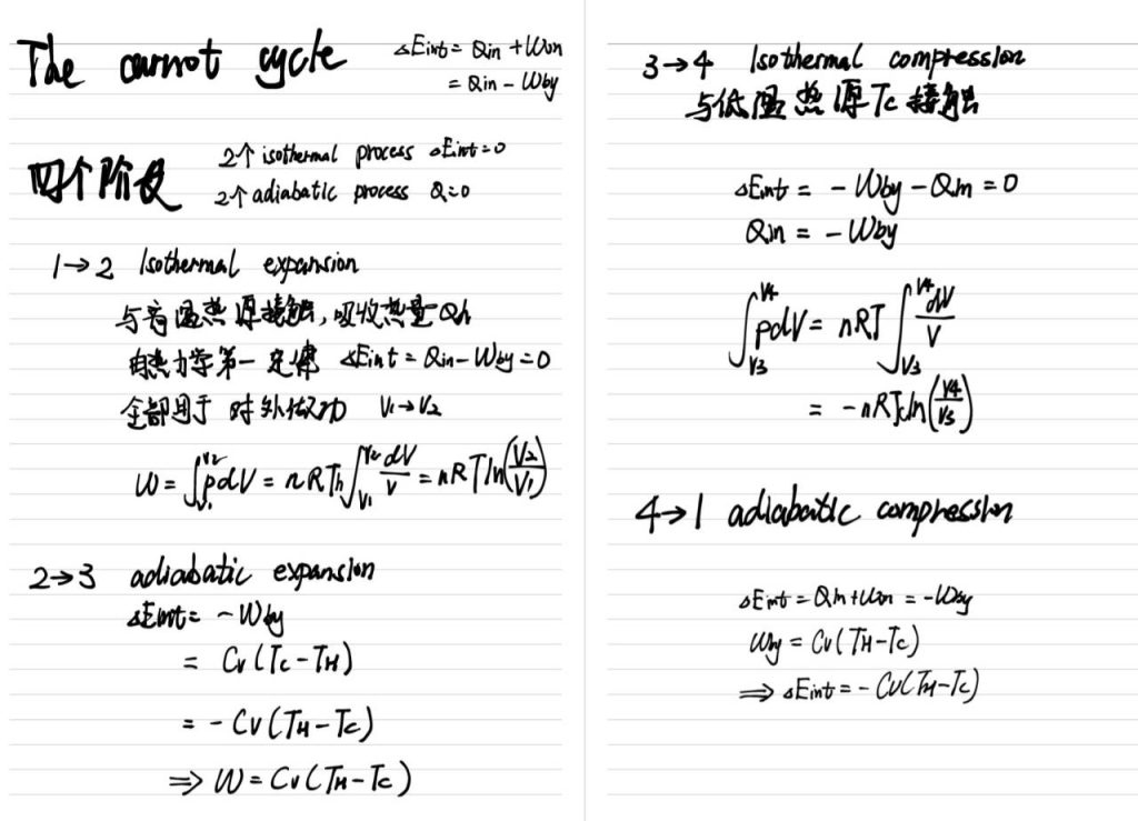
coefficient of performance

$$COP = \frac{T_c}{T_h – T_c}$$

在热机反向运行（如制冷机或热泵）的情境下，COP用于衡量系统的效率，具体物理含义为：系统从低温热源吸收的热量与运行过程中所消耗能量的比值.

COP 定义差异源于对不同系统中 “有用热量” 的界定：制冷系统关注从低温热源提取的 $Q_C$，供热系统关注向高温热源添加的$Q_h$.

Entropy

Entropy is a measure of the microscopic randomness associated with a closed system.

Irreversible process

• General Heat engine efficiency

卡诺循环的最大效率依赖于 “可逆性”；为了更精确地描述过程的可逆程度，需要引入一个新参数 —— 熵，它用于量化过程的可逆性.

由于卡诺循环是可逆循环，在可逆过程中，$\Delta S_{\text{总}}=0$，即系统与外界的总熵变之和为零；因此，高温热源减少的熵等于低温热源增加的熵，即高温热源失去的熵完全转移给了低温热源.

$$\eta’=1-\frac{Q_c’}{Q_h’}$$

• Inequality of efficiencies

$\eta’\leq \eta$，即$1-\frac{Q_c’}{Q_h’}\leq 1-\frac{T_c}{T_h}$

即$\frac{T_c}{T_h}\leq \frac{Q_c’}{Q_h’}\Rightarrow \frac{Q_c’}{T_c’}-\frac{Q_h’}{T_h}\geq0$

Clausius theorem

• For a cycle

$$ \Delta S_{res} = -\oint \frac{dQ}{T} \geq 0 $$

• For a process

$$ \Delta S = \int \frac{1}{T} dQ_{rev} $$

Partial Differentiation

Function of Multiple Variables

total Derivative

当函数所有变量都发生变化，且变量间存在依赖关系，全导数$\frac{dw}{dx}=(\frac{\partial{w}}{\partial{u}})_v\frac{du}{dx}+(\frac{\partial{w}}{\partial{v}})_u\frac{dv}{dx}$

Partial Derivative

• 定义

固定其它变量，仅对其中一个变量求导

• 应用场景

用于分析多元函数中单一变量对结果的影响，如热力学中固定体积$V$，研究内能$U$随温度$T$的变化率$(\frac{\partial{U}}{\partial{T}})_V$

Properties

• symmetry of the second derivatives

$$\left( \frac{\partial}{\partial v} \left( \frac{\partial w}{\partial u} \right)_v \right)_u = \left( \frac{\partial}{\partial u} \left( \frac{\partial w}{\partial v} \right)_u \right)_v$$

Also can be written as:

$$\frac{\partial^2 w}{\partial u \partial v} = \frac{\partial^2 w}{\partial v \partial u}$$

在多元函数的偏导数分析中，函数 $f(x, y)$ 的值可以作为一个变量来处理。

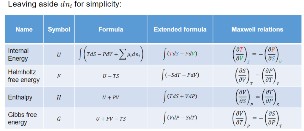
Thermodynamic Potentials, Chemical Potential and Enthalpy

Thermodynamic Potentials

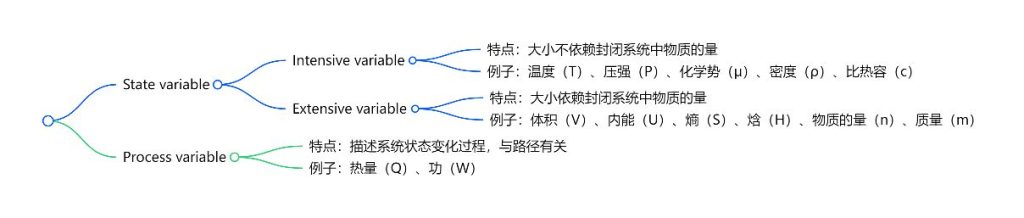
• Intensity variable: the magnitude does not depend on the amount of substance in a closed system.

• Extensive variable: the magnitude depends on the amount of substance present in a closed system

Fundamental Thermodynamic Relation

We have been writing the first law as:

$$\Delta U = Q_{in} + W_{on}$$

But the differential form is of more use (small changes, integrable)

$$dU = dQ_{in} + dW_{on}$$

For a \underline{reversible process}, we have that:

$$dS = \frac{dQ_{rev}}{T} \quad dW_{on} = -P dV$$

And so:

$$dU = T dS – P dV$$

where $ U, S, V $ are state variables! Properties of the material, not the process. This also holds for non – reversible processes.

$$\boxed{dU = T dS – P dV}$$

• chemical potentials

如果存在化学反应，以上公式就遗漏了一个用于解释分子数量变化的项；分子携带能量，因此若不是封闭系统，则必须考虑这部分能量.

$$ dU = TdS – PdV + \sum_{i} \mu_{i} dn_{i} $$

Where $\mu_{i}$ are the $\underline{\text{chemical}\ \text{potentials}}$ of particles of type $i$ and $dn_{i}$ is the number of them. We are literally counting the numbers of molecules and the chemical energy they hold.

$$ dU = TdS – PdV + \sum_{i} \mu_{i} dn_{i} + \sum_{j} X_{j} dx_{j} $$

Thermodynamic Potentials and Free Energy

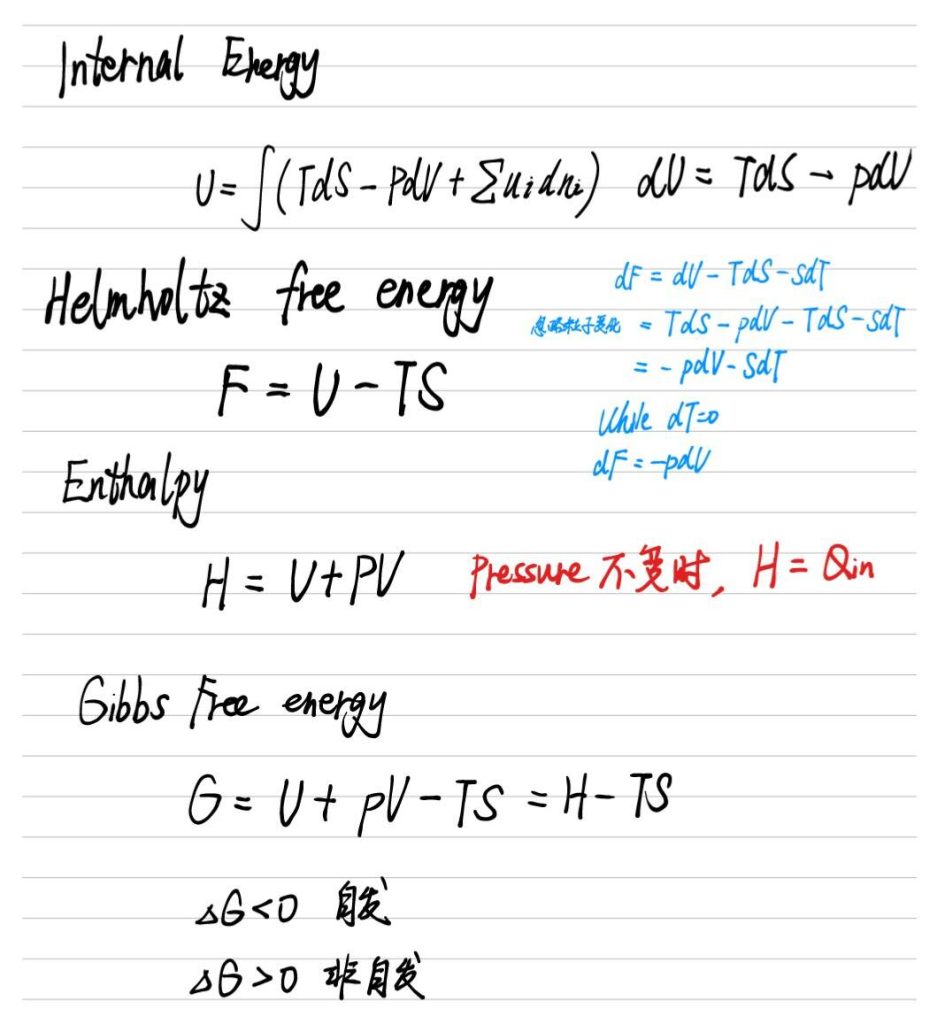
Thermodynamic Potentials and Maxwell Relations

Relativity