数学中最神奇的函数就是$e^x$了.

基本微积分

积分

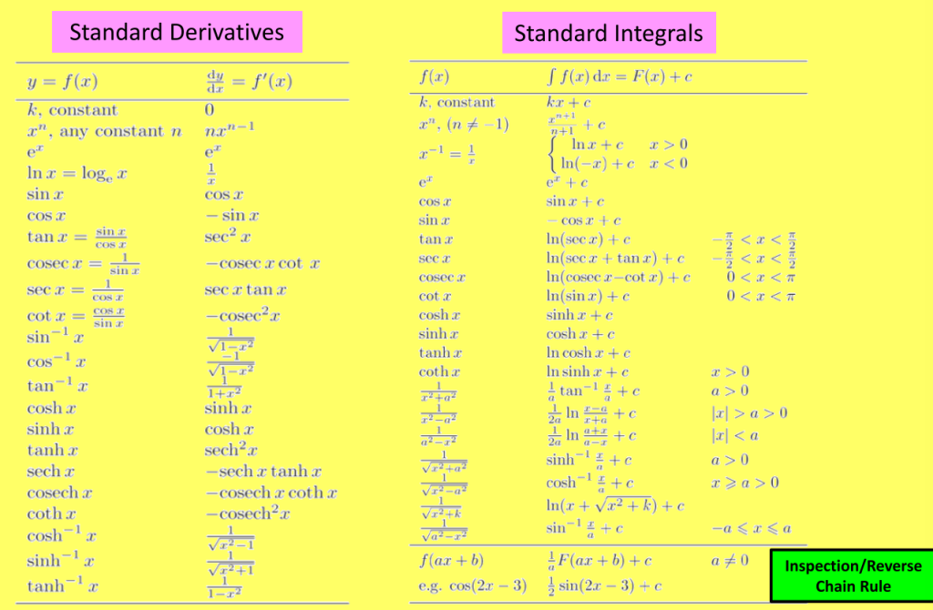
Standard Derivatives/Integrals

Integration of Parametric Equations

$$\int ydx=\int y \frac{dx}{dt}dt$$

这个等式展示了积分变量替换的原理，尤其是在处理参数方程的情形下.
之所以要引入$dt$，是由于有$y=f(t)$，并不为了别的什么.
这种替换常用于参数方程的积分问题，比如计算曲线下的面积或物理中的功.

hyperbolic trig function

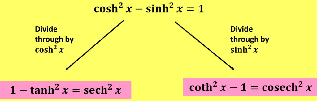
三角函数基于单位圆，平方和为1；而双曲函数则是基于双曲线，平方差为1.

$$\cosh^2x-\sinh^2x=1$$

Reciprocal hyperbolic function

$$ \text{sech} x =\frac{1}{\cosh x}=\frac{2}{e^x+e^{-x}}$$

$$\text{cosech} x =\frac{1}{\sinh x}\frac{2}{e^x-e^{-x}}$$

$$\coth x =\frac{1}{\tanh x}\frac{e^{2x}+1}{e^{2x}-1}$$

Hyperbolic Identities

Standard Integrals

---

微分方程

$1^{st}$ Order ODE

A linear $1^{st}$ order differential equation in standard form is:

$$ \frac{dy}{dx}+P(x)y=Q(x) $$

可分离变量法

Reverse Product Rule

$$f(x)\frac{dy}{dx}+yf'(x)=g(x)$$

观察到式中两部分存在原函数和导数关系，就能将两部分合并起来：

$\frac{d}{dx}(yf(x))=g(x)$ so that $yf(x)=\int g(x)dx$.

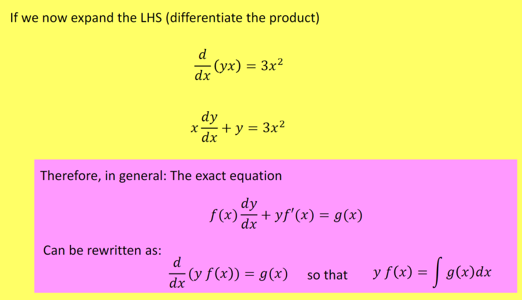
What we are doing is using the product rule backwards so that both sides can be easily integrated.

Integrating factor

As we know, the integrating factor is given by:

$$ e^{\int P(x)dx} $$

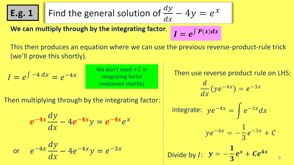
• STEP 1: Divide by anything on front of 𝑑𝑦/𝑑𝑥

“Standard form” means that the coefficient of $\frac{dy}{dx}$ is 1.

• STEP 2: Determine integrating factor, 𝐼
• STEP 3: Multiply through by 𝐼 and use product rule backwards
• STEP 4: Integrate and simplify
• STEP 5: Divide by 𝐼

Substitution Method (Homogeneous)

A Homogeneous differential equation is of the form: $\frac{dy}{dx}=f(x,y)$.

Where $f(x,y)$ is a homogeneous function of degree $n$. That is $f(kx,ky)=k^nf(x,y)$ for any non-zero constant $k$.

$k$用来检验方程是否属于homogeneous differential equation，通过将$x,y$替换为$kx,ky$，计算$f(kx,ky)$是否可以替换为$k^nf(x,y)$.

Homogeneous $2^{nd}$ order ODEs

Complementary equation

• Second order：未知函数的最高阶导数是二阶导数
• Linear：未知函数及其导数的最高次幂都是一次的，并且没有未知函数与其导数的乘积项
• Constant coefficients：未知函数$y$及其导数的系数都是常数

二阶线性常系数微分方程的general form：

$$a\frac{d^2y}{dx^2}+b\frac{dy}{dx}+cy=f(x)$$

特别地，当$f(x)=0$时，该方程为二阶线性齐次常系数微分方程.

对于线性齐次方程：

若$g(x)$是解答，那么$Cg(x)$也是方程的解.

如果$g(x)$和$h(x)$均为方程的解，那么$(g(x)+h(x))$也是方程的解；同理，$(C_1g(x)+C_2h(x))$也是方程的解.

Chracteristic equation

https://www.youtube.com/watch?v=SPVqgkOZMAc

求解二阶齐次微分方程 $y” + 5y’ + 6y = 0$:

假设解的形式为 $y = e^{rx}$，则：

\begin{aligned}
y’ &= r e^{rx}, \\
y” &= r^2 e^{rx}.
\end{aligned}

将 $y$、$ y’ $、$ y” $ 代入原方程：

\begin{aligned}
r^2 e^{rx} + 5r e^{rx} + 6e^{rx} &= 0, \\
e^{rx}(r^2 + 5r + 6) &= 0.
\end{aligned}

因为 $e^{rx} \neq 0 $，所以特征方程为：
$$
r^2 + 5r + 6 = 0
$$

分解因式：
$$
(r + 2)(r + 3) = 0
$$
解得 $r = -2 $或 $r = -3 $.

因此，方程的通解为：
$$
y = C_1 e^{-2x} + C_2 e^{-3x}.
$$

最重要的过程就在于假设未知函数的结构，即以下这一步：

$y=e^{rx}$

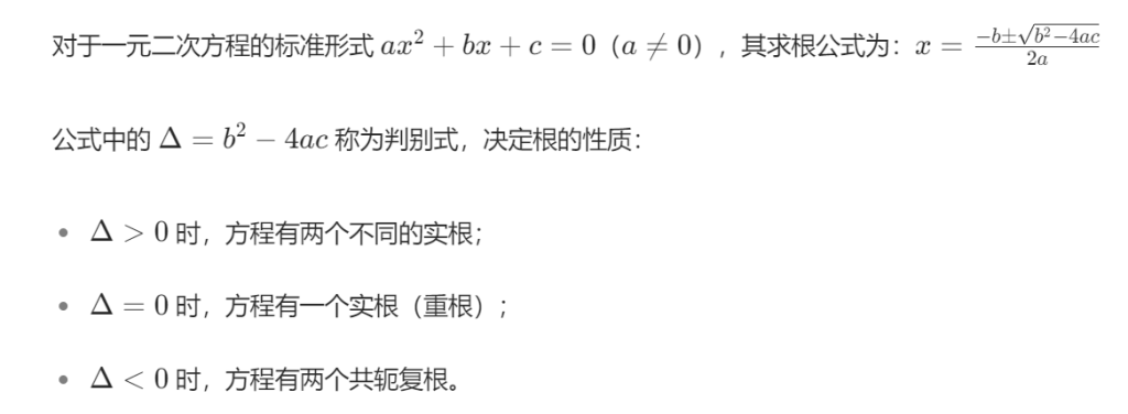
解决这种二阶线性齐次微分方程的问题，实际上就是解一元二次方程的问题.

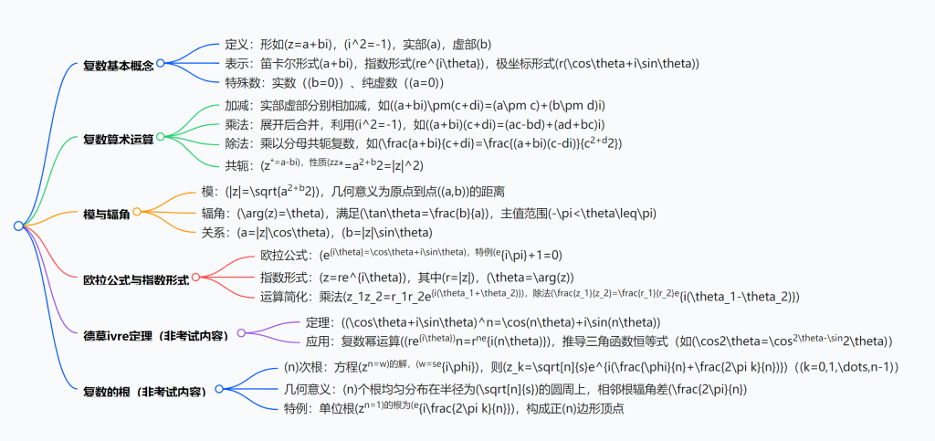
复数

\begin{aligned}
z=&a+bi\\ =&\sqrt{a^2+b^2}e^{i\tan^{-1}\left(\frac{b}{a}\right)} \\ =&re^{i\theta}
\end{aligned}

卡西欧991CN计算负数

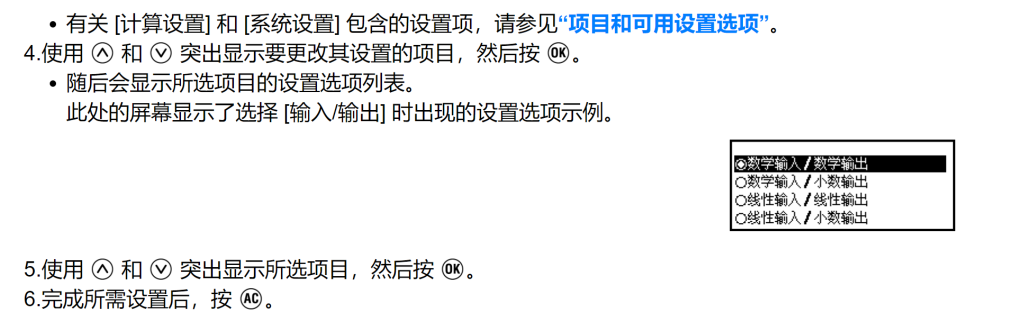
在设置中调整数学输入/数学输出，以输出无理数结果.

菜单中选择复数模式，ENG打出i.

Modulus and Argument

笛卡尔形式转换为极坐标形式

对于复数$z=a+bi$，其中$Re(z)=a$，$Im(z)=b$：

\begin{aligned}
&r = \sqrt{a^2+b^2}\\
&\theta = tan^{-1}\left(\frac{b}{a}\right)
\end{aligned}

将$a=r\cos\theta$，$b=r\sin\theta$代入复数的笛卡尔形式$z=a+bi$可得：

$$z=r(\cos\theta+i\sin\theta)$$

辐角的取值范围

根据复数在复平面上的位置，$\text{arg}(z)$的取值范围需要进行调整，通常有：

\begin{aligned}
-\pi<\text{arg}(z)\leq \pi
\end{aligned}

Euler’s Formula

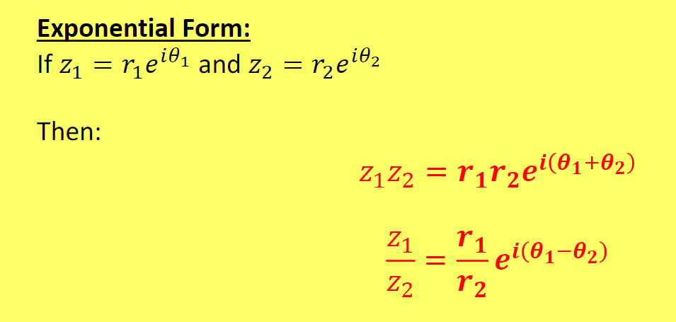
Exponential Form

\begin{align*} e^{i\theta} &= 1 + i\theta + \frac{(i\theta)^2}{2!} + \frac{(i\theta)^3}{3!} + \frac{(i\theta)^4}{4!} + \cdots \\ &= 1 + i\theta – \frac{\theta^2}{2!} – \frac{i\theta^3}{3!} + \frac{\theta^4}{4!} + \cdots \\ &= \left(1 – \frac{\theta^2}{2!} + \frac{\theta^4}{4!} – \cdots \right) + i \left( \theta – \frac{\theta^3}{3!} + \frac{\theta^5}{5!} – \cdots \right) \\ &= \cos \theta + i \sin \theta. \end{align*}

由此可以使用通过欧拉公式转化后的指数形式复数简化计算：

向量

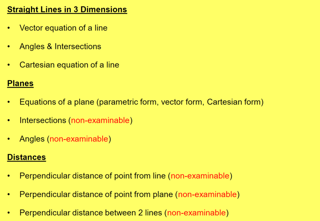
• 直线向量方程
  $$\mathbf{r} = \mathbf{a} + \lambda \mathbf{d}$$
  $\mathbf{a}$ 为已知点，$\mathbf{d}$ 为方向向量）
• 平面点法式方程
  $$\mathbf{r} \cdot \mathbf{n} = d$$
  $\mathbf{n}$ 为法向量，$d = \mathbf{a} \cdot \mathbf{n}$
• 平面参数方程
  $$\mathbf{r} = \mathbf{a} + \lambda \mathbf{u} + \mu \mathbf{v}$$
  $\mathbf{u}, \mathbf{v}$ 为平面内方向向量
• 点到平面距离
  $$\frac{|\mathbf{p} \cdot \mathbf{n} – d|}{|\mathbf{n}|}$$
  $$\frac{|ax_p + by_p + cz_p – d|}{\sqrt{a^2 + b^2 + c^2}}$$
• 两直线夹角
  $$\cos \theta = \frac{|\mathbf{d}_1 \cdot \mathbf{d}_2|}{|\mathbf{d}_1||\mathbf{d}_2|}$$
• 两平面夹角
  $$\cos \theta = \frac{|\mathbf{n}_1 \cdot \mathbf{n}_2|}{|\mathbf{n}_1||\mathbf{n}_2|}$$
• 叉积求法向量
  $$\mathbf{n} = \overrightarrow{AB} \times \overrightarrow{AC}$$
  适用于三点确定平面

向量基础运算

Dot Product / Scalar Product

定义

$$ a \cdot b = | a | | b |\cos\theta$$

关键性质

• 交换律：$(a \cdot b = b \cdot a)$
• 垂直向量：若$ (a \perp b)$，则 $(a \cdot b = 0)$
• 投影（Projection）：$a 在b 方向的投影为 (\frac{a \cdot b}{|b|})$

Cross Product / Vector Product

Triple Products

Scalar Triple Product

Vector Triple Product

formula sheet上有

直线的向量方程

三维直线

$$r=a+\lambda d$$

其中$a$为线上已知点，$d=a-b$为方向向量，$\lambda$为参数

• Parallel lines
• Intersecting lines
• Perpendicular lines
• Skew lines

Angles between straight lines

$$\cos\theta = \frac{d_1\cdot d_2}{|d_1 ||d_2 |}$$

计算两条直线的夹角只使用了方向向量部分，而没有使用基准点的数据.

Cartesian form

向量方程转换为笛卡尔方程，核心就是先分别找到三个方向的向量方程（从每个方向单独解出参数$\lambda$），联立消去参数即可.

If $a= \begin{pmatrix} a_1 \\ a_2 \\ a_3 \end{pmatrix} $ and $d = \begin{pmatrix} d_1 \\ d_2 \\ d_3 \end{pmatrix} $ and $r = \underline{a} + \lambda \underline{d} $ is the equation of straight line, then its Cartesian form is$ \frac{x – a_1}{d_1} = \frac{y – a_2}{d_2} = \frac{z – a_3}{d_3} $.

平面的向量方程

$$r=a+\lambda u + \mu v$$

若只有方向向量$\boldsymbol{u}$ 和 $\boldsymbol{v}$（描述平面的延展方向），而没有$\boldsymbol{a}$，则只能表示过原点的平面.

当$\boldsymbol{a}$ 改变时，会得到与之平行的其他平面，形成 “平行平面族”；因此，$\boldsymbol{a}$ 是确定唯一平面的关键 —— 如同直线方程中基准点确定直线位置，$\boldsymbol{a}$ 让平面在空间中有了确切的 “位置锚点”.

平面的法向量

若平面的参数方程为$r=a+\lambda u+\mu v$，取方向向量$u$和$v$，法向量为：
$$n=u\times v$$

矩阵

Matrix Fundamentals

A matrix with only one column is called a column vector or column matrix.

• A matrix with only one column is called a column vector or column matrix.

For example,\begin{pmatrix} 1 \ 2 \ 3 \end{pmatrix} \begin{pmatrix} x_1 \ x_2 \ x_3 \end{pmatrix} are both $3 \times 1$ column vectors/matrices.

• A matrix with only one row is called a Row vector or Row matrix.

For example,$ (-1 \quad 2 \quad 2 \quad 0)$ is a $ 1 \times 4$ row vector/matrix.

The distributive law

$$k(A+B)=k A+k B$$

Where $k$ is a scalar.

Matrix Multiplication

• 卡西欧操作

菜单 – 4【矩阵】- OPTN – 定义矩阵

• Matrix Multiplication involving \mathbf{I}

For any square matrix $\mathbf{A}$ and identity matrix $\mathbf{I}$ of the same size,
$$\mathbf{AI} = \mathbf{IA} = \mathbf{A}$$

(algebra equivalent $a \times 1 = 1 \times a = a$)
(multiplying by $I$ on the left or right leaves the original matrix unchanged)

• Properties

Order is important, in general, $$\mathbf{AB} \neq \mathbf{BA}$$ (not commutative)

Multiplication is associative $$\mathbf{(AB)C = A(BC)}$$

Order is important, but placement of brackets isn’t.

Multiply out brackets as usual $$\mathbf{A(B + C) = AB + AC}$$

Powers $$\mathbf{A^2 = AA, A^3 = AA^2}\ \text{or}\ \mathbf{A^2A}$$

Zero Matrix $$\mathbf{AB = \underline{0}}$$ does not mean that $\mathbf{A = 0}, \mathbf{B = 0}$ (the product could just result in zeroes for every element)

Multiplying with transposes $$\mathbf{A^TA}$$ and $$\mathbf{AA^T}$$ are always possible and the result is symmetric $$\mathbf{(AB)}^T = \mathbf{B}^T\mathbf{A}^T$$ (order is changed) $$\mathbf{A}^T\mathbf{A}^T = (\mathbf{A}^T)^2 = (\mathbf{A}^2)^T$$ (using last result)

Verification of these are left as tutorial exercises.

Gaussian Elimination

Elementary Row Operations

• Row Interchange
  We can swap rows around.
• Row Scaling
  We can multiply a row (or rows) by a scalar constant.
• Row Addition/Subtraction
  This is exactly what we do when we use the elimination method in simultaneous equations (hence the name).

主要用途是对增广矩阵进行化简和消元.

Forming the Augmented Matrix

Given we may need to do multiple row operations, for $\underline{notational convenience}$, we can write the matrix equation $ \mathbf{A}x = \mathbf{b} $ as an \underline{augmented matrix} ($ \mathbf{A}|\mathbf{b} $)

Row-Echelon Form

增广矩阵通过初等行变换将左下角的数消去为0，得到pivot.

pivot

On each row, the left-most non-zero entry, known as the leading entry or pivot, is to the right of the leading entry in the row above.

Suppose we have used row operations to reduce a matrix and have obtained:

\begin{pmatrix} 2 & 3 & -2 & | & 1 \\ 0 & 0 & 7 & | & 0 \\ 0 & -6 & 4 & | & 6 \end{pmatrix}

This is not in row echelon form as the pivot in row 2 is zero. However, we can just switch row 2 and 3

\begin{pmatrix} 2 & 3 & -2 & | & 1 \\ 0 & -6 & 4 & | & 6 \\ 0 & 0 & 7 & | & 0 \end{pmatrix}

Which is now in the correct form and easily solvable.

Solutions

• Infinite Solutions
  通过行变换将其中一行所有元素均消为0，无法确定其中一个未知数的具体值；此时任意选取一个未知数，令$x_{random}=k$，从而表示其它未知数.
• No Solutions

处理增广矩阵后得到如$0x_3=4$等明显不成立的情况，则方程组无解.

The Transpose of a Matrix

Transposing the transpose gives back the original matrix: $(\mathbf{A}^{\mathbf{T}})^{\mathbf{T}} = \mathbf{A}$.

For identity matrix $\mathbf{I}$, the transpose has no effect: $\mathbf{I}^{\mathbf{T}} = \mathbf{I}$

我的理解：转置就是将matrix逆时针转动90°

If $\mathbf{A}$ is an $m \times n$ matrix, $\mathbf{A}^{\mathbf{T}}$ is an $n \times m$ matrix.

Properties of the Transpose

$$(\mathbf{A} + \mathbf{B})^{\mathrm{T}} = \mathbf{A}^{\mathrm{T}} + \mathbf{B}^{\mathrm{T}}$$

$$(\mathbf{A} – \mathbf{B})^{\mathrm{T}} = \mathbf{A}^{\mathrm{T}} – \mathbf{B}^{\mathrm{T}}$$

$$(\mathbf{A}^{\mathrm{T}})^{\mathrm{T}} = \mathbf{A}$$

The Determinant

The determinant is also a convenient way to work out vector products.

对于二元一次方程组

\begin{cases}
ax + by = e \\
cx + dy = f
\end{cases}

其系数矩阵 $\mathbf{A} = \begin{pmatrix}a & b \\ c & d\end{pmatrix}$，行列式为 $\det(\mathbf{A}) = ad – bc$：

• 当 $\det(\mathbf{A}) \neq 0$，方程组有唯一解
• 若 $\det(\mathbf{A}) = 0$，解的情况为无解或无穷多解

The Inverse Matrix

Matrices can be thought of as a function that can transform a point.

The determinant of a matrix $\mathbf{A} = \begin{pmatrix} a & b \\ c & d \end{pmatrix}$ is
$ \det(\mathbf{A}) = |\mathbf{A}| = \begin{vmatrix} a & b \\ c & d \end{vmatrix} = ad – bc $
Product of forward diagonals minus product of backward diagonals.

• If $ \det(\mathbf{A}) = 0 $, then $\mathbf{A}$ is a singular matrix and it does not have an inverse.
• If $ \det(\mathbf{A}) \neq 0 $, then $\mathbf{A}$ is a non – singular matrix and it has an inverse.

Properties of Inverse Matrices

$ \mathbf{A}^{-1}\mathbf{A} = \mathbf{I} $

$ (\mathbf{A}^{\text{T}})^{-1} = (\mathbf{A}^{-1})^{\text{T}}$

$ (\mathbf{AB})^{-1} = \mathbf{B}^{-1}\mathbf{A}^{-1} $

$ (\mathbf{A}^{-1})^{-1} = \mathbf{A} $

$ (k\mathbf{A})^{-1} = \frac{1}{k}\mathbf{A}^{-1} $

$ (\mathbf{ABC})^{-1} =\mathbf{C}^{-1}\mathbf{B}^{-1}\mathbf{A}^{-1} $

Eigenvalues & Eigenvectors

An eigenvector $\mathbf{u}$ of a matrix $\mathbf{A}$ is a non – zero vector that remains unchanged in direction by the transformation：

$\mathbf{A}\mathbf{u} = \lambda\mathbf{u}$.

$\lambda$ (the scaling factor) is known as the \underline{eigenvalue} of the eigenvector $\mathbf{u}$.

Eigenvector

矩阵 $A$ 代表一种线性变换，它对大多数向量的作用是同时改变其方向和长度；但特征向量 u 具有特殊性：在 $\mathbf{A}$ 的作用下，它的方向（或反向，当 $\lambda < 0$ 时）保持不变，仅长度按比例 $|\lambda|$ 缩放；这种 “方向不变性” 使 $\mathbf{u}$ 成为特殊的向量，它揭示了矩阵 $\mathbf{A}$ 所代表变换的一种 “固有方向”，是矩阵 $\mathbf{A}$ 内在特性的体现.

The characteristic equation

$$ \det(\mathbf{A} – \lambda\mathbf{I}) = 0 $$

Examples to follow：

1. Form the matrix $\mathbf{A} – \lambda\mathbf{I}$

2. Use (3) to form the characteristic polynomial and solve to find the eigenvalues.

3. Use (2) to find the corresponding eigenvector for each eigenvalue.